RTT Under Load: A Beginner's Tour Through 30 iperf3 Tests
Get link
Facebook
X
Pinterest
Email
Other Apps
Packets & Patterns
Notes from a second-year CSE student on how networks actually behave
RTT Under Load: A Beginner's Tour Through 30 iperf3 Tests
Computer Networks — Digital Assignment | BCSE308L | VIT Chennai 24BCE5047 | Naman Bhukar | Slot: F1+TF1 | Dr SubbuLakshmi T
If you have ever run ping google.com and watched the numbers, you have already met RTT — Round Trip Time, the time it takes for a packet to travel from your machine to a destination and come back. Most of us treat RTT as a fixed property of a link: "my ping to this server is about 250 ms, done."
That intuition is wrong. The goal of this post is to show you why, using real measurements from 30 iperf3 tests run against iperf.he.net, captured with Wireshark and plotted. The short version: RTT is not a number your network has. It is a number your network produces — and it depends heavily on how busy that network is right now.
The Test Setup
All tests were run from the same machine against the same server (iperf.he.net, Hurricane Electric's public iperf3 endpoint), on the same link, back-to-back. The 30 runs were grouped into three traffic classes:
Low traffic (L1–L10): 1 stream, small or capped data rates, short durations. Think "normal browsing."
Medium traffic (M1–M10): 2–3 parallel streams, moderate bandwidth, longer durations. Think "a few Zoom calls plus a download."
High traffic (H1–H10): 5–10 parallel streams, or UDP floods at 50–200 Mbps. Think "maximum stress."
For each run, RTT samples were extracted from the TCP timestamps in the packet capture. What we are looking at is essentially the network answering one question, thousands of times per second: "If I send a packet right now, how long will a reply take?"
The Big Picture First
Before digging into individual tests, here are the two summary charts — they give you the 10-second version of the entire story.
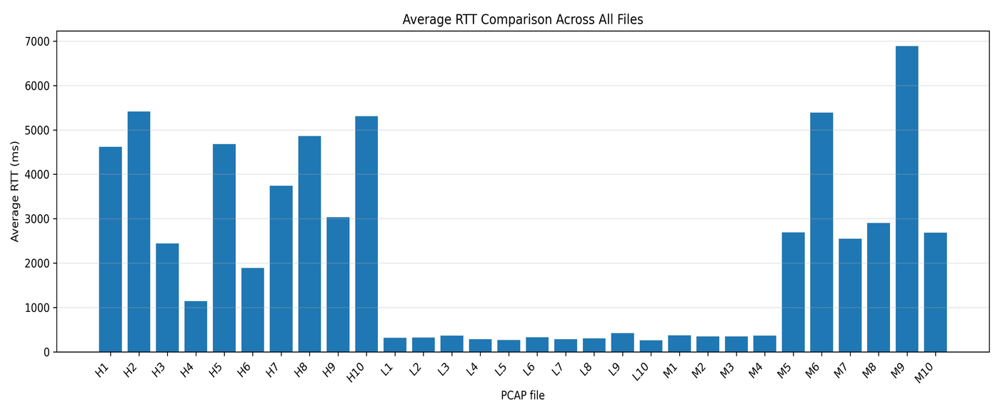
Figure 1 — Average RTT across all 30 runs, grouped by traffic class.
Inference. The L bars (low traffic) are barely visible — all hover near the 250–400 ms baseline. The M bars split into two distinct groups: M1–M4 look like L-tests, but M5–M10 jump to multi-second averages. The H bars are uniformly large, with H2 and H10 pushing above 5000 ms. The single most striking observation is that M9 (6886 ms) beats every high-traffic test except one — meaning "medium" is not always milder than "high." Traffic shape matters more than traffic volume.
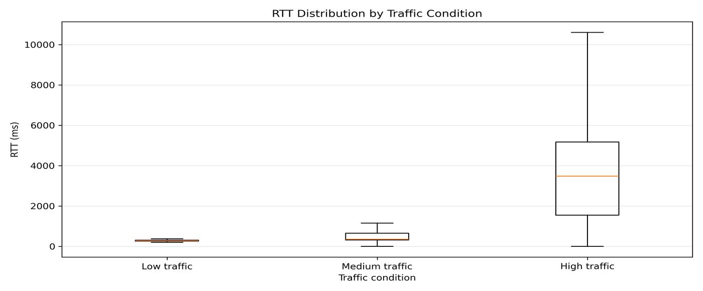
Figure 2 — Boxplot of RTT samples grouped by traffic condition.
Inference. Low traffic is a tight, flat box near the baseline — the RTT barely varies. Medium traffic is slightly higher but still compact at the median, with a longer upper tail. High traffic is a completely different animal: the box itself stretches from roughly 1500 ms to 5200 ms, with a whisker reaching past 10000 ms. This single chart is the headline: network load does not shift RTT by a constant — it stretches the distribution exponentially.
Headline numbers
Traffic class
Typical average RTT
Worst sustained run
Worst spike observed
Low (L1–L10)
~258–423 ms
L9: 423 ms
~16 s (teardown)
Medium (M1–M10)
~346 ms – 6886 ms
M9: 6886 ms
~18 s
High (H1–H10)
~1143 ms – 5416 ms
H2: 5416 ms
~31 s
The baseline RTT on this link — the best case, when the network is idle — sits around 250–260 ms. That is the physical floor: the speed-of-light-plus-switching cost of a round trip from India to the Hurricane Electric server. Nothing we do can make it lower. But as the rest of this post shows, we can make it vastly higher.
Stage 1 — Low Traffic (L1–L10)
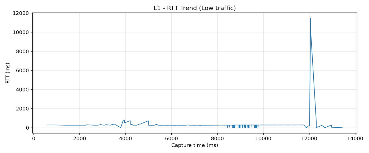
The low-traffic tests are the reference point. One TCP stream, short durations, sometimes with bandwidth caps (-b) or tiny send buffers (-l). These runs answer the question: "what does RTT look like when the network is not stressed?"
Inference. RTT sits almost flat at ~280–320 ms across the entire 10-second test. The single 11-second spike near the 12 s mark is a TCP connection teardown artefact, not congestion. Average RTT is 318 ms with a standard deviation of 304 ms — almost all of that std-dev comes from the one spike. This is what "a calm network" looks like.
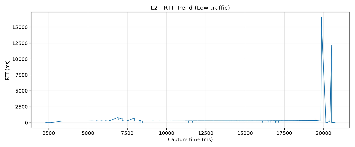
Inference. Nearly identical behaviour to L1 — RTT hugs the baseline for the entire measurement window, with end-of-capture spikes that are again teardown noise. Average 324 ms, very close to L1. Increasing the test duration from 10 s to 15 s changed essentially nothing: with only one stream and no rate cap, TCP never pushes hard enough to build queues.
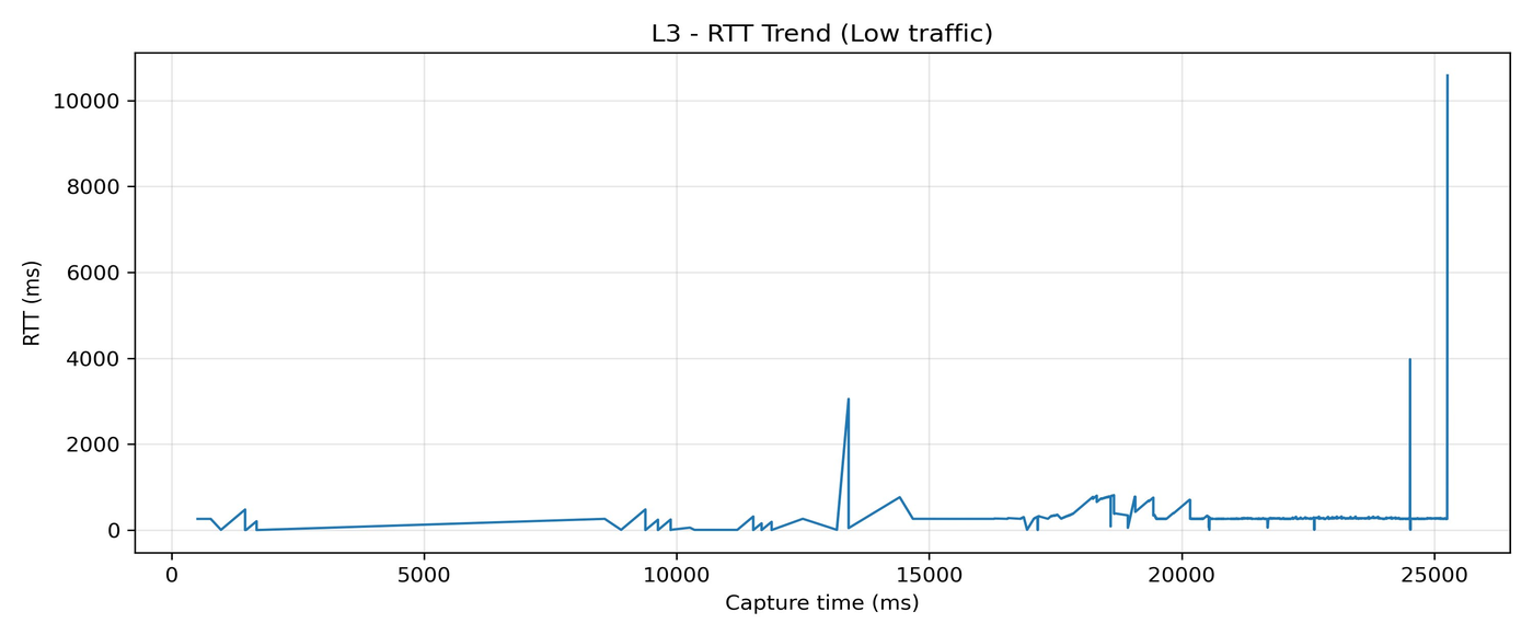
Inference. Same flat profile stretched to 25 seconds of capture. One mid-test spike of ~3 s around 13 s is a transient path event, but the line returns to baseline almost immediately. Average 364 ms. The takeaway: duration alone — without changing the load shape — does not push RTT around.
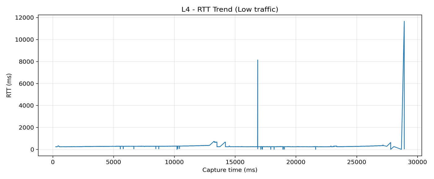
Inference. The longest single-stream test, and the most stable: average RTT 283 ms with a standard deviation of just 105 ms — the lowest variance of any L-test. When TCP has time to settle into a steady state on a lightly loaded link, it produces extremely predictable latency.
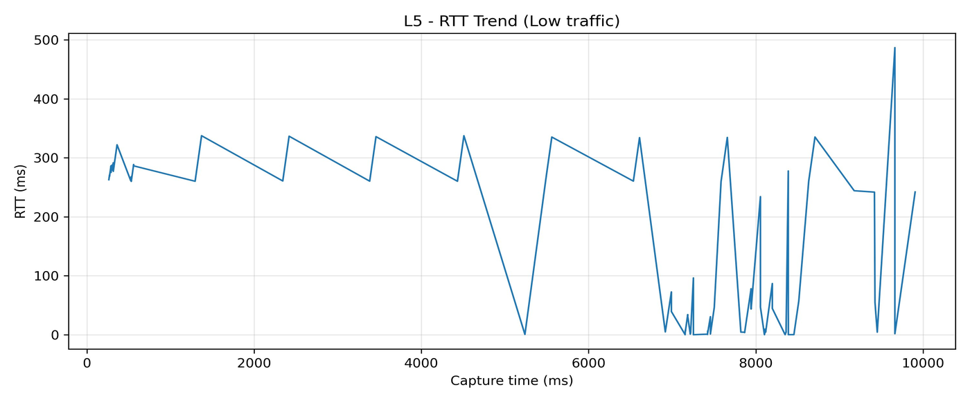
Inference. A faint sawtooth pattern between ~260 ms and ~340 ms in the first 5 seconds. That shape is TCP's pacing loop made visible — the 1 Mbps rate cap is slow enough that each queue-fill-and-drain cycle shows up distinctly. Average stays low at 266 ms.
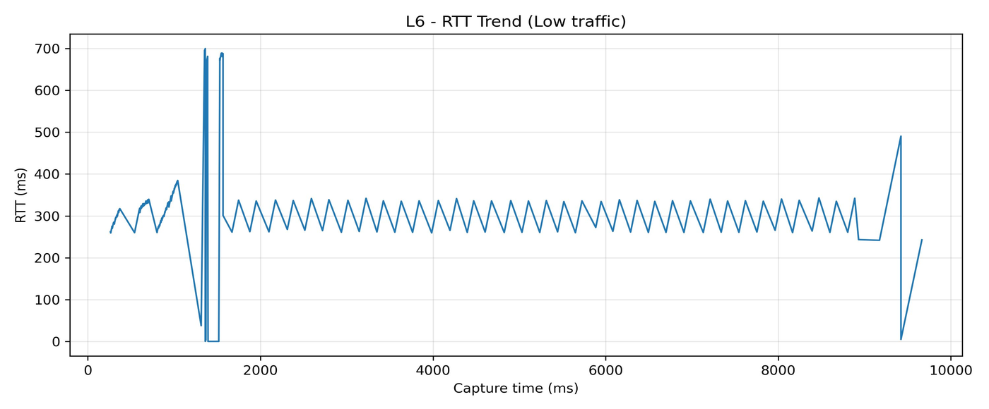
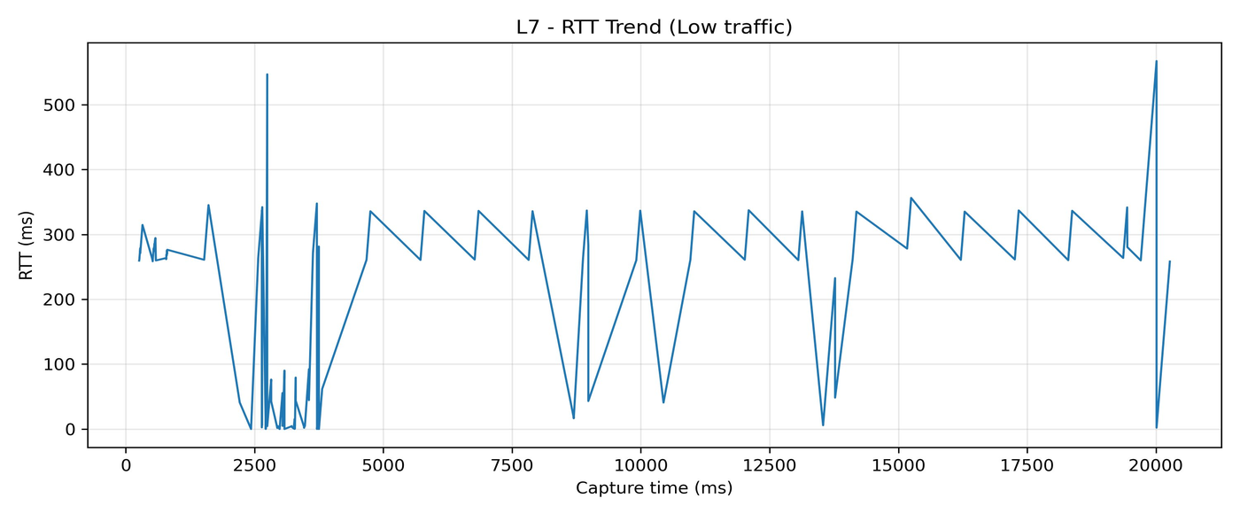
Inference. The clearest sawtooth in the whole dataset. RTT oscillates between ~260 ms and ~340 ms, roughly 40 cycles across the 10-second window. This is TCP's congestion control breathing in slow motion: queue fills → RTT rises → sender backs off → queue drains → RTT falls → repeat.
Inference. L7 is L5 extended to 20 seconds. Average RTT 283 ms, std-dev only 62 ms — the second tightest distribution in the entire dataset. Rate-capped low traffic is the most predictable network state we observe.
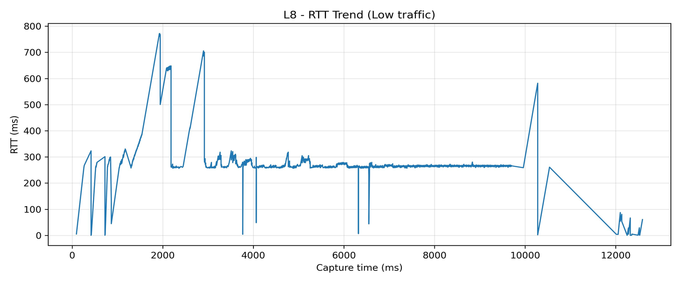
Inference. RTT spikes to 500–770 ms in the first 3 seconds before settling back to baseline. A 128-byte buffer means roughly 10× more packets per second to move the same data — more packets-per-second equals more queueing work everywhere along the path.
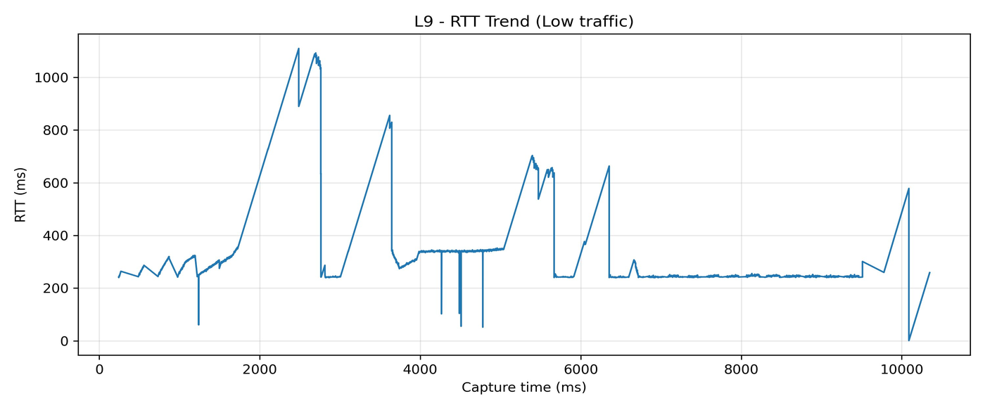
Inference. The most dramatic low-traffic run. RTT climbs in waves to over 1100 ms before TCP throttles back. Average RTT 423 ms — the highest of any L-test. Buffer size matters: how you send data is almost as important as how much.
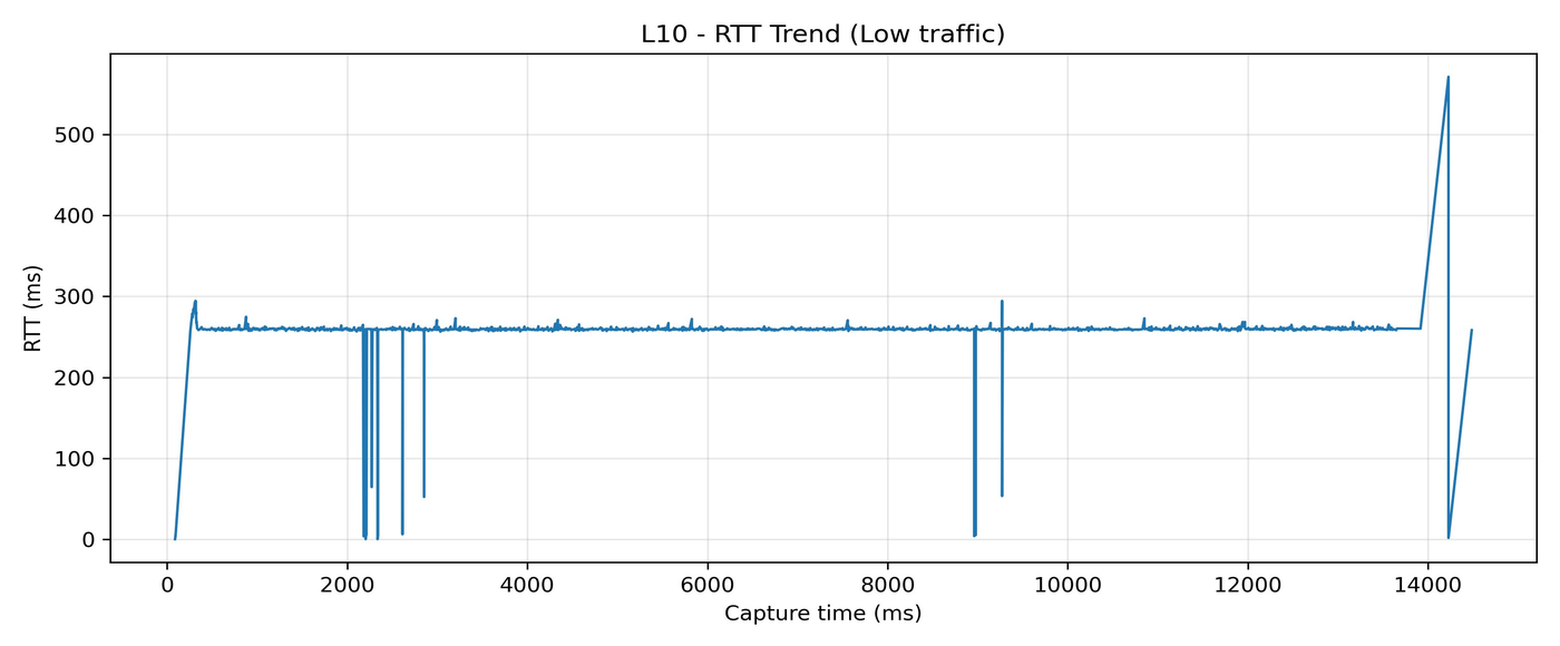
Inference. The quietest run in the entire dataset: average 258 ms, std-dev just 23 ms. The 2 Mbps cap prevents the buffer size from causing damage. Rate-pacing beats small-buffer amplification when both are present.
Stage 2 — Medium Traffic (M1–M10)
This is where the story turns surprising. You would expect "medium" to behave like a mild version of "high." It does not. Medium traffic splits into two very different camps, and recognising them is the most important lesson in this entire post.
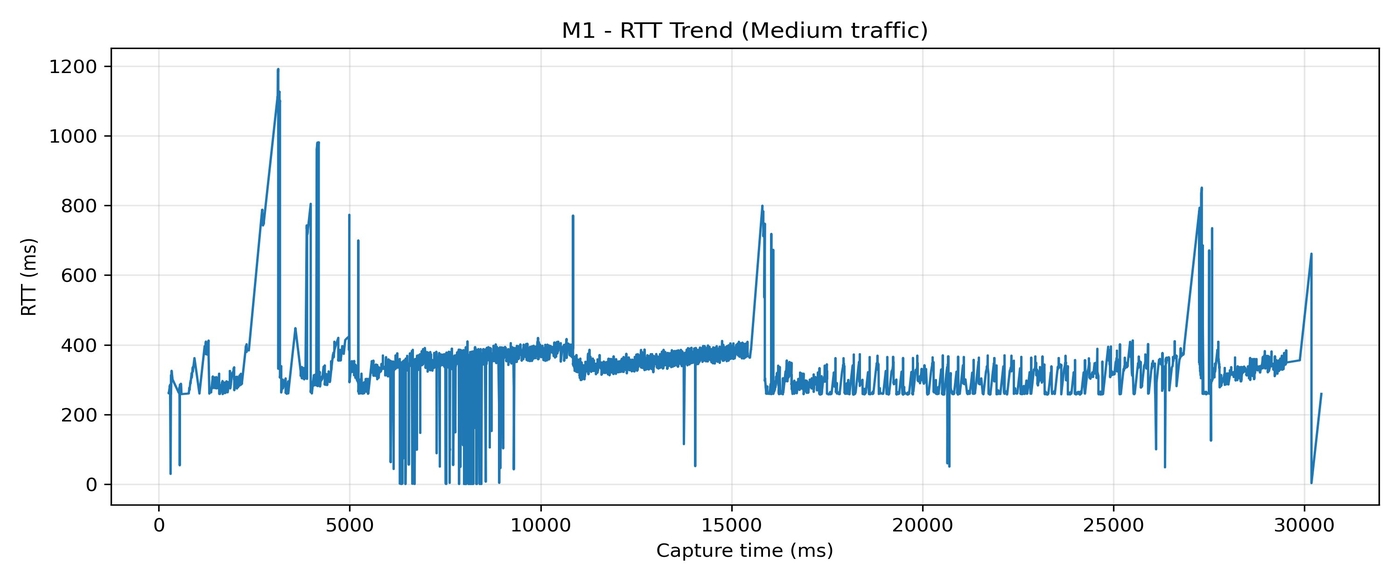
Inference. Two parallel streams, no cap, 30 seconds. Average RTT 371 ms — essentially the same as a low-traffic test. Adding a second stream barely moved the needle.
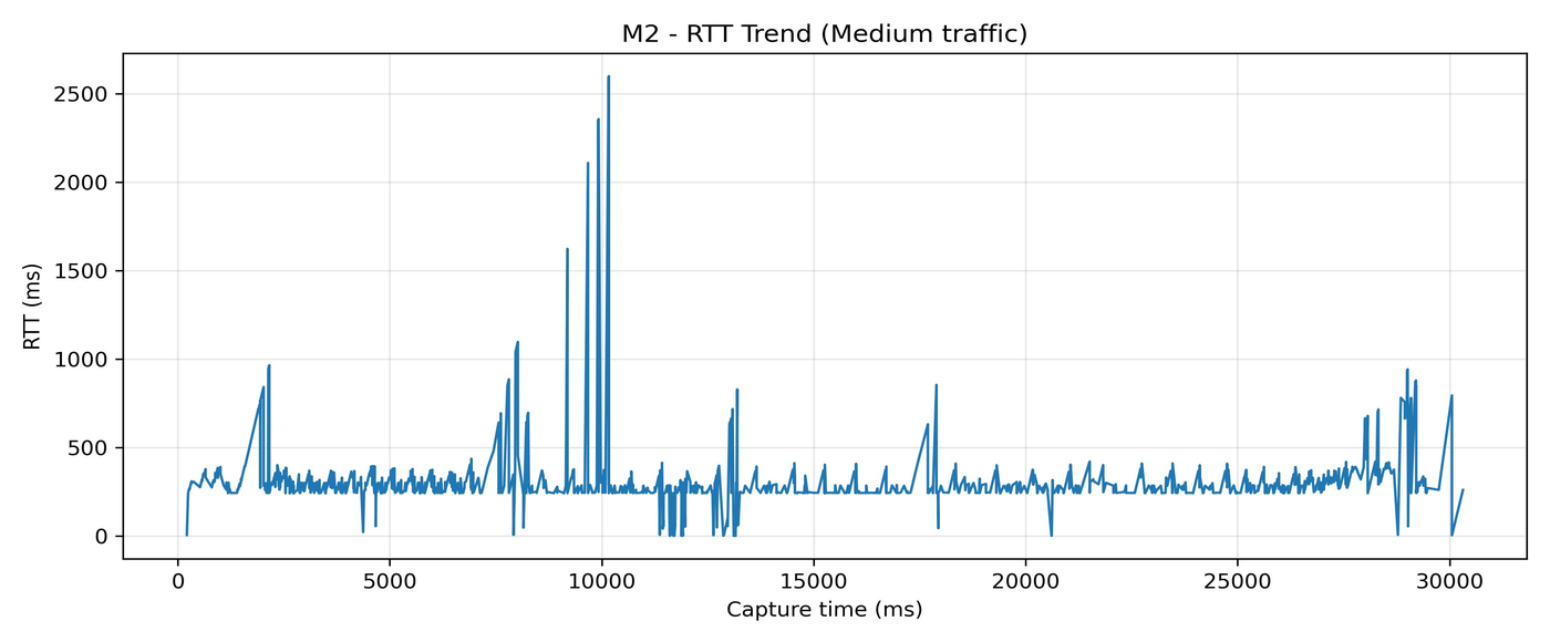
Inference. Three streams, 30 seconds. Average 348 ms, even lower than M1. Tripling the stream count without a rate cap produced essentially no RTT increase.
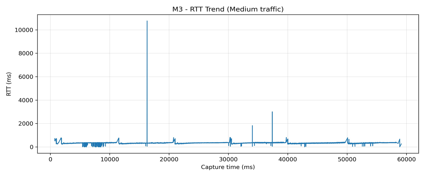
Inference. 2 streams for a full minute. Average 346 ms, std-dev only 84 ms. When TCP is allowed to self-regulate, it keeps queues small even across many parallel flows.
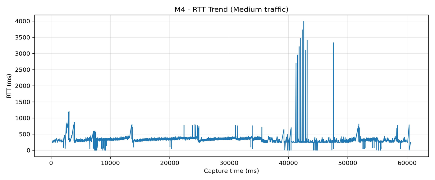
Inference. Three streams over a full minute. Average 363 ms. M1–M4 form "Camp A": unpaced parallel TCP, staying near baseline because TCP's feedback loop is intact.
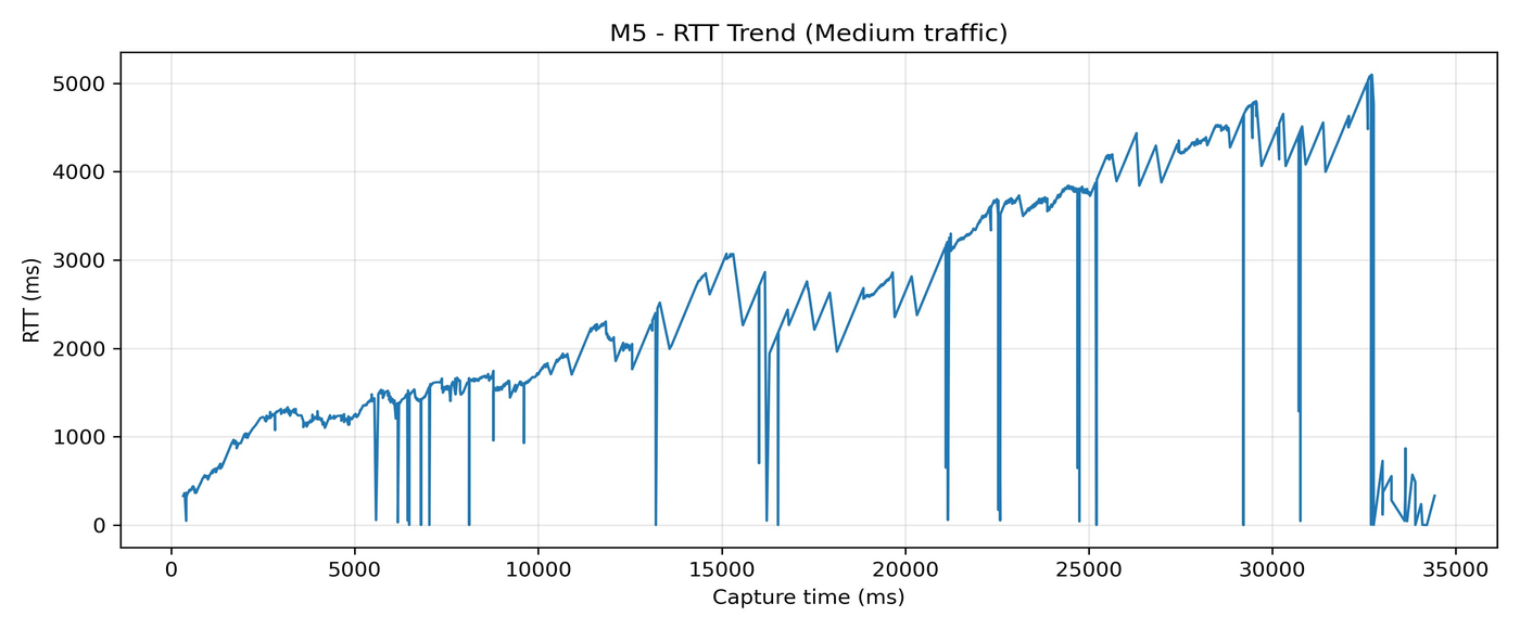
Inference. RTT climbs in a slow, relentless ramp from 300 ms to over 5000 ms across the 30-second run. Average 2692 ms. This is bufferbloat, and it is the single most important pattern in the post.
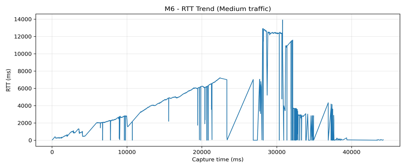
Inference. The cap doubles and the damage doubles. RTT ramps to ~7000 ms by the 23 s mark. Average 5391 ms — higher than most high-traffic tests. The higher cap fills the queues faster and pushes them further past their comfortable operating point.
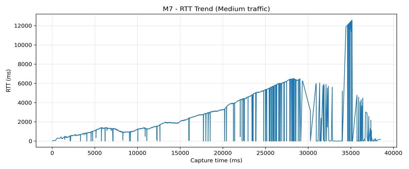
Inference. A textbook bufferbloat ramp: smooth, almost linear climb to ~5500 ms by the 33 s mark. Average 2901 ms. Once a run enters the bufferbloat regime, the curve takes on a recognisable signature regardless of the specific parameter that triggered it.
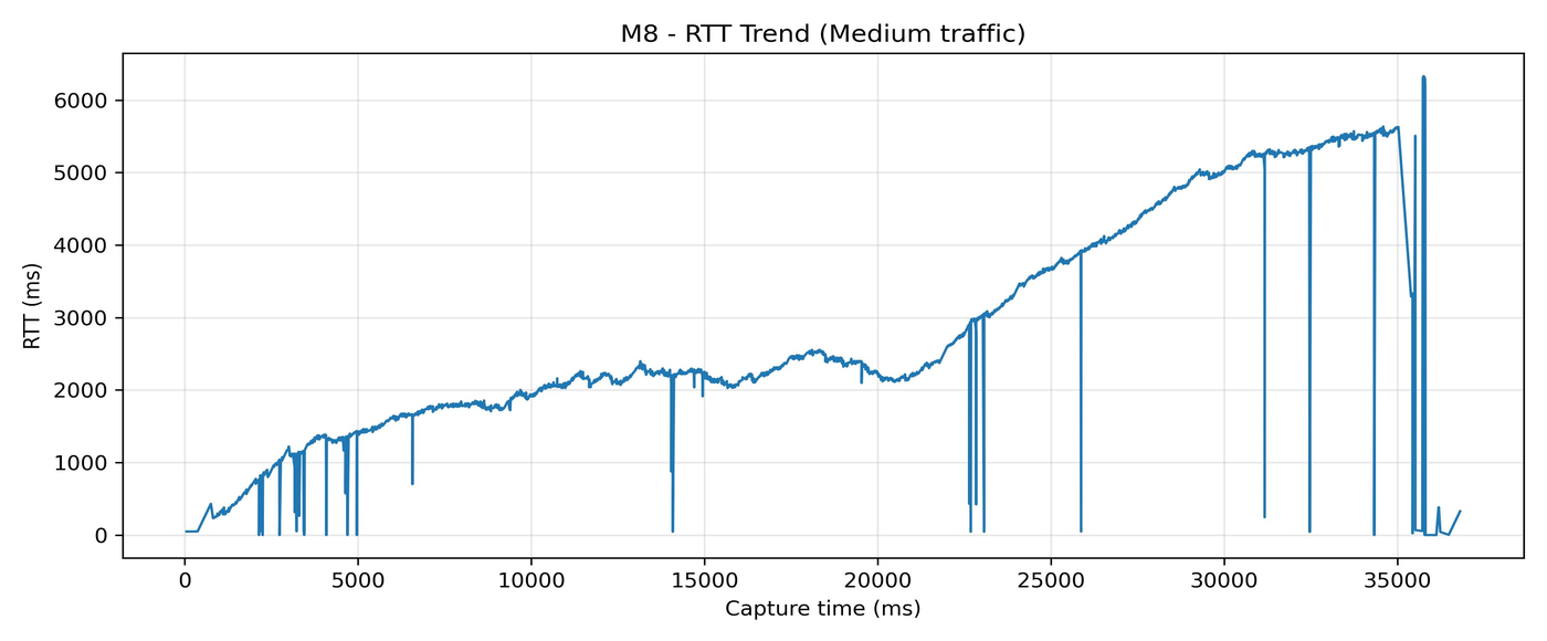
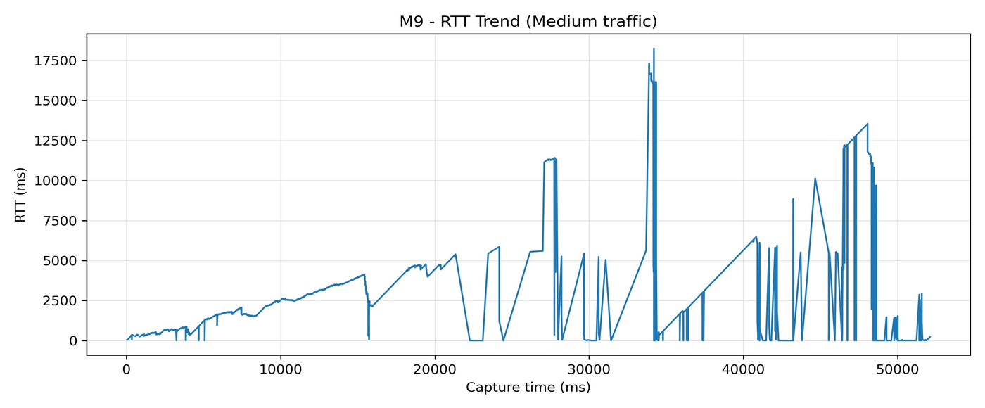
Inference. The worst RTT average in the entire dataset: 6886 ms. Only 2 streams, but a 15 Mbps cap and a long 45-second window give the queues plenty of time to fill. M9 beats every high-traffic test on average RTT.
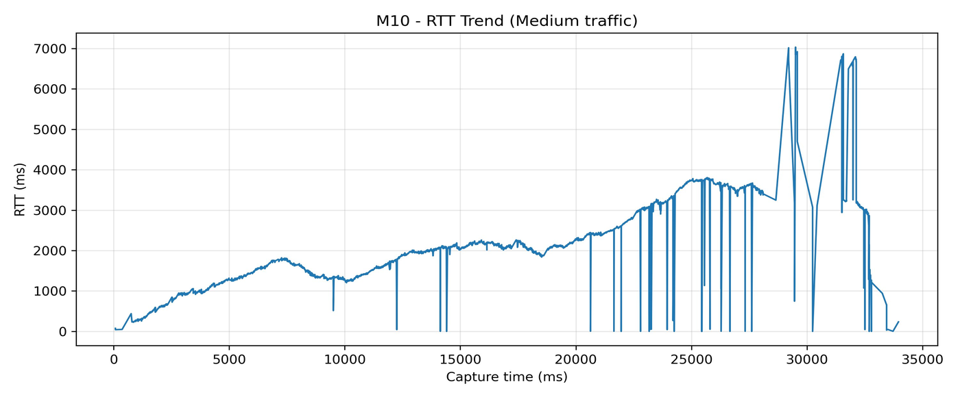
Inference. Average 2681 ms. Interestingly less severe than the simpler M9. The right single parameter at the right magnitude can do more damage than three parameters combined.
Stage 3 — High Traffic (H1–H10)
Now the "obvious" bad case: 5–10 parallel TCP streams, or UDP floods at tens to hundreds of megabits per second.
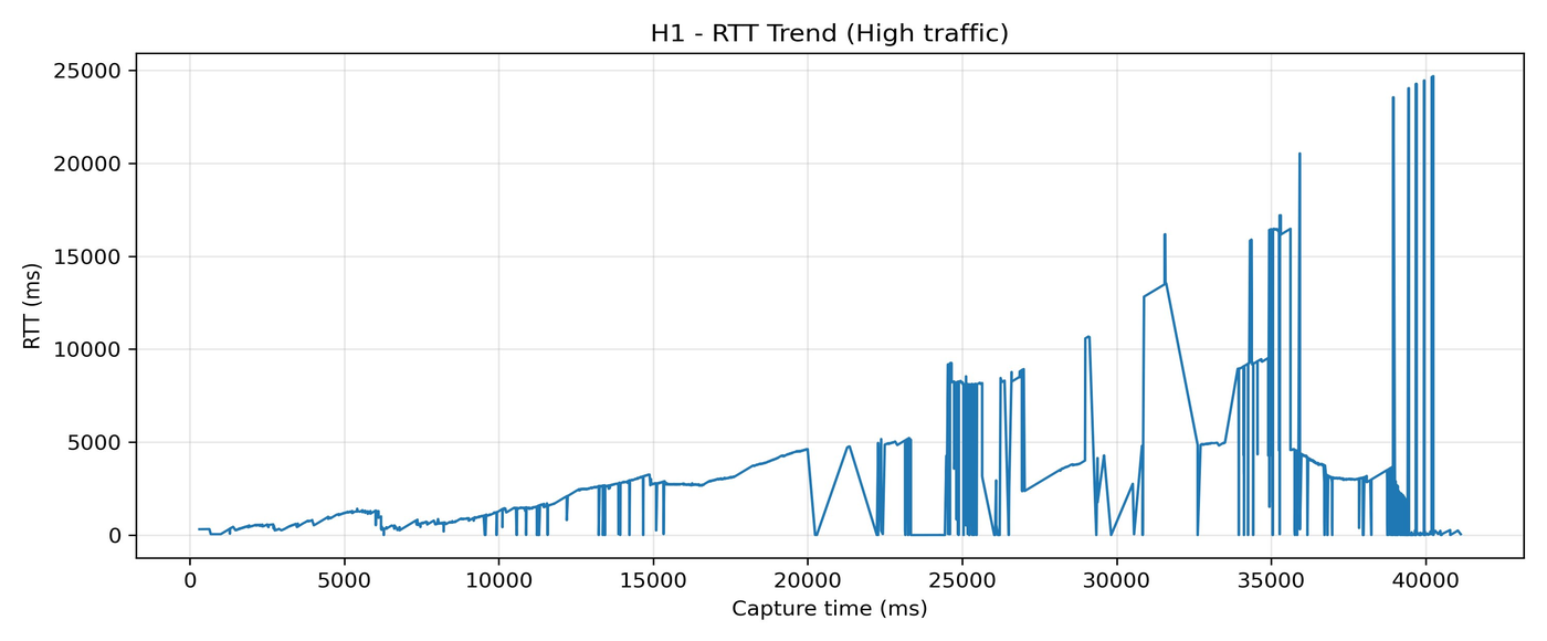
Inference. RTT starts near 300 ms, ramps steadily, hits ~5000 ms at the halfway mark, then turns chaotic with spikes to 24 seconds at the tail. Average 4617 ms — roughly 15× the baseline.
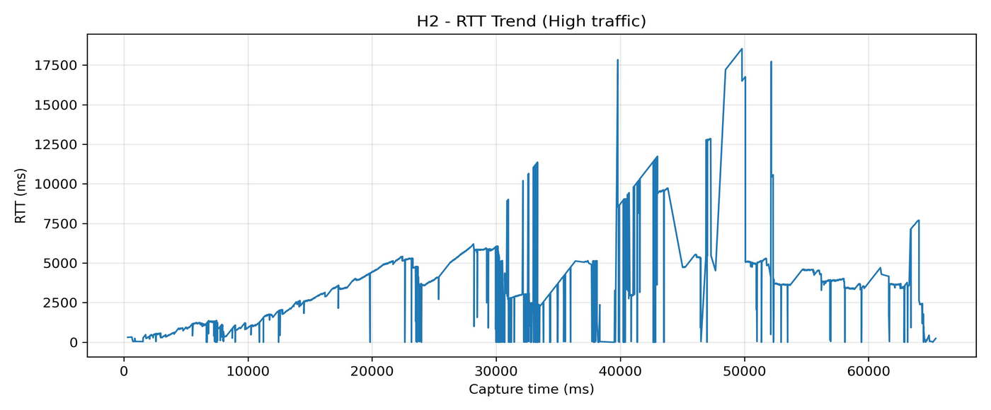
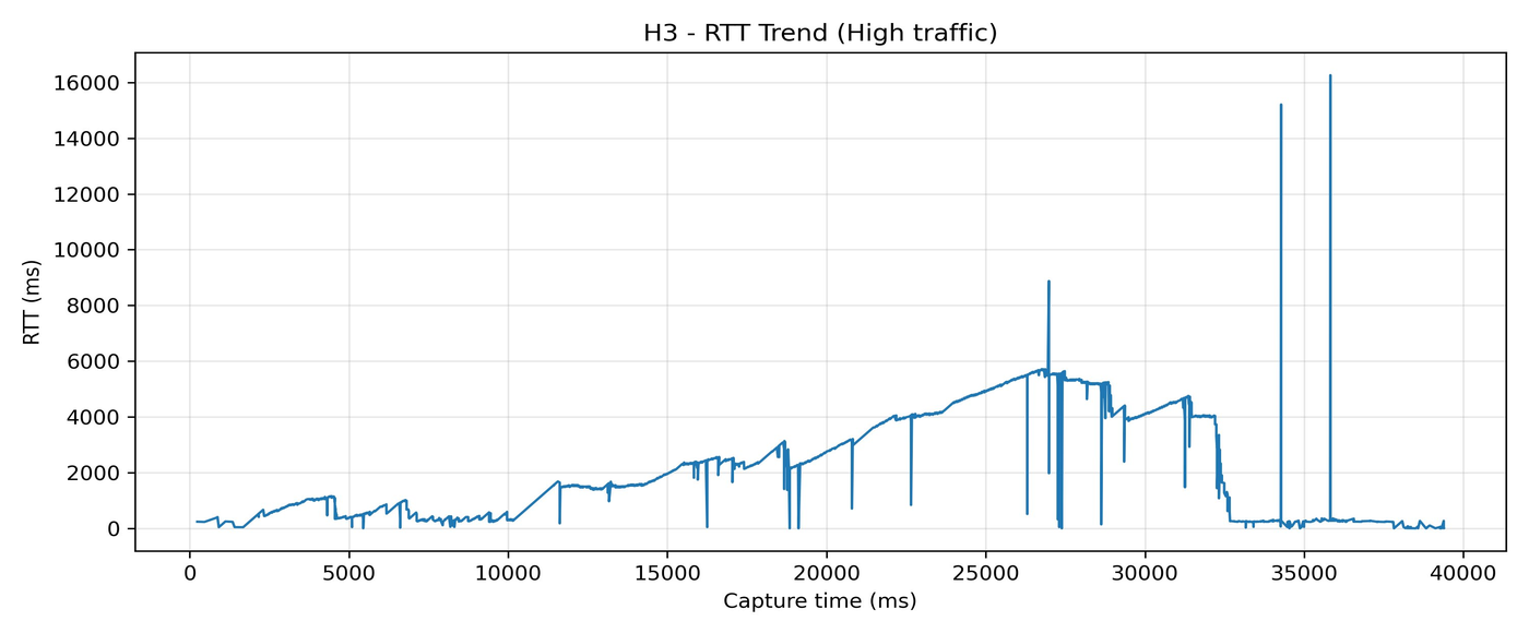
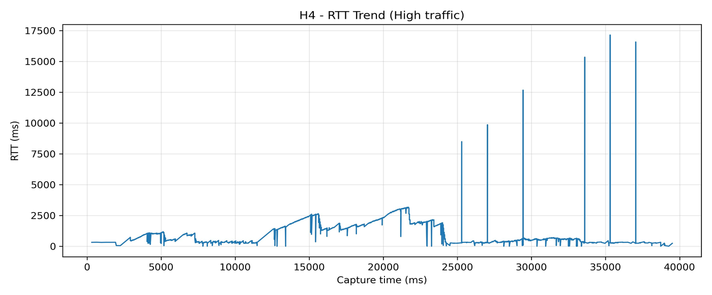
Inference. Eight streams, 30 seconds. Average drops to 2439 ms — better than H1 despite more streams. With more parallel flows, TCP's congestion control fires more often, keeping individual queues from running away.
Inference. Ten streams and the best TCP-high-traffic result: average 1143 ms. Counter-intuitive but real: more streams can produce lower average RTT than fewer streams.
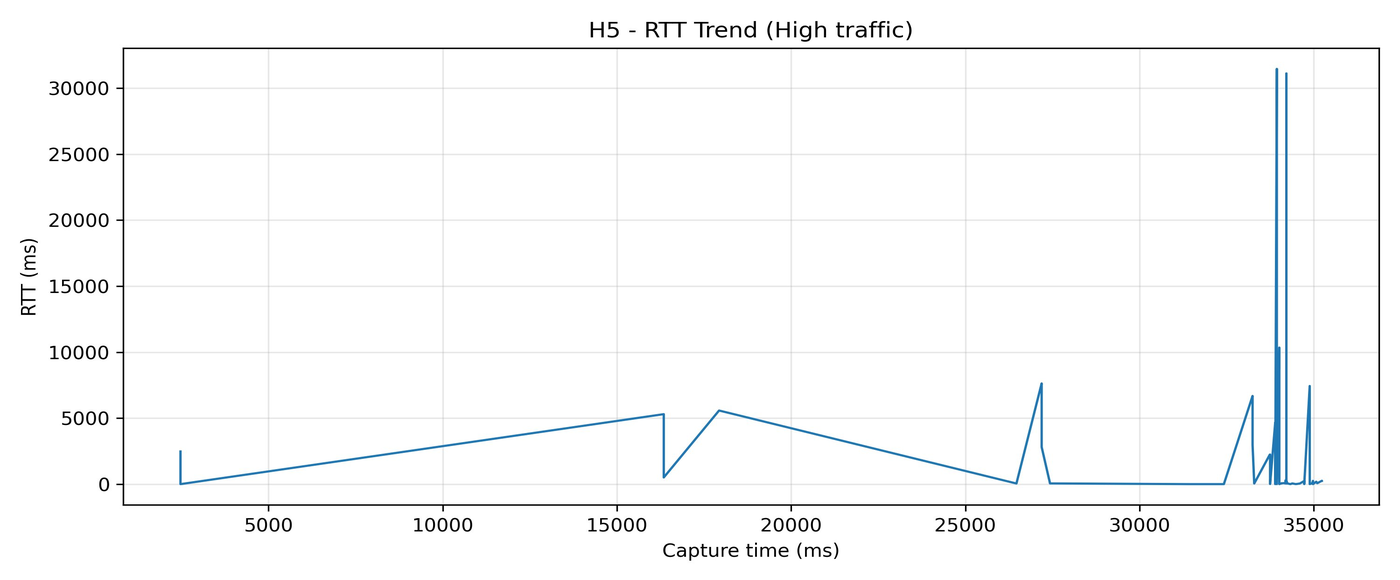
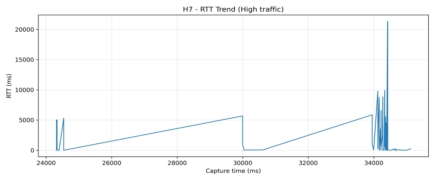
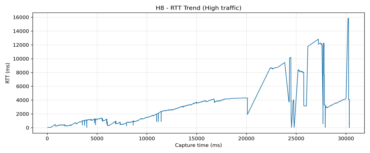
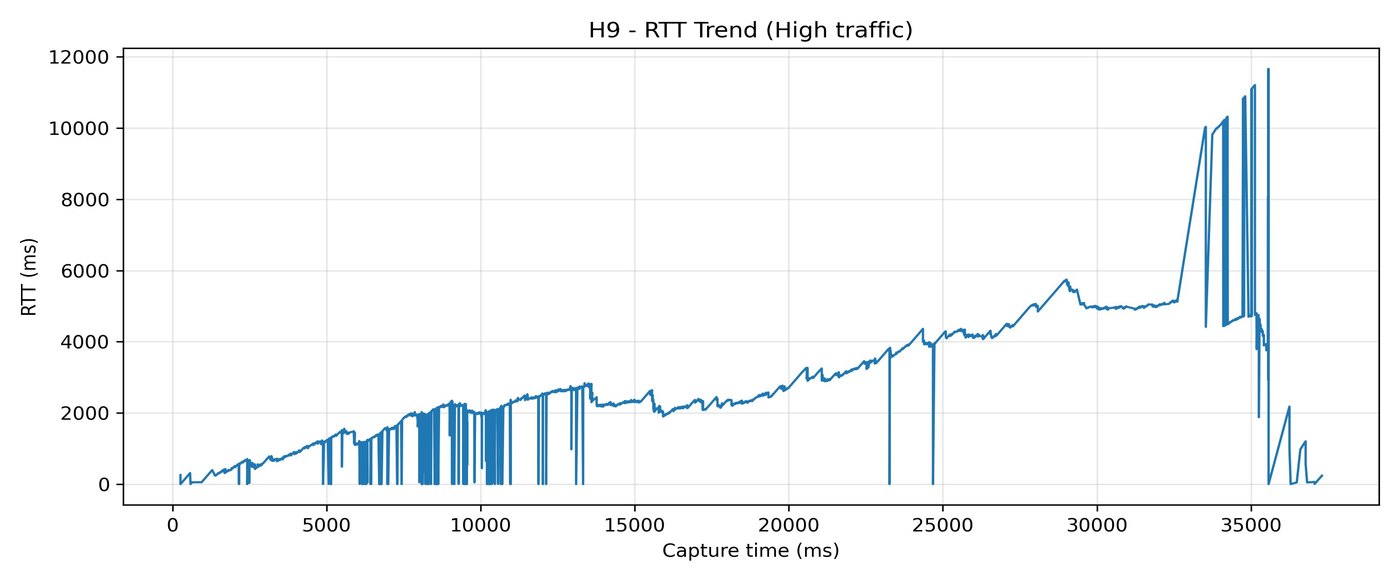
Inference. A long, almost perfectly linear ramp from 0 up to ~5500 ms over 13 seconds, then a collapse, then another ramp. UDP has no congestion control — pure queue-fill, queue-overflow, queue-reset cycles.
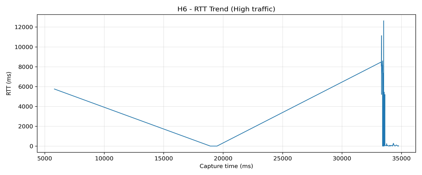
Inference. The cleanest UDP triangle in the set. Average 1888 ms — lower than H5 despite doubled bandwidth, because the 100 Mbps rate produces fewer RTT samples. Protocol behaviour is visible in the shape of the curve.
Inference. At 200 Mbps only 169 RTT samples survive the capture. Average 3739 ms, but the number is unreliable — what we are really measuring is a link that has been knocked out of normal operation. UDP without pacing is how you DDoS yourself.
Inference. Average 3031 ms. Large buffers actually help: fewer packets-per-second means less per-packet queueing overhead, and a smoother ramp shape compared to H8.
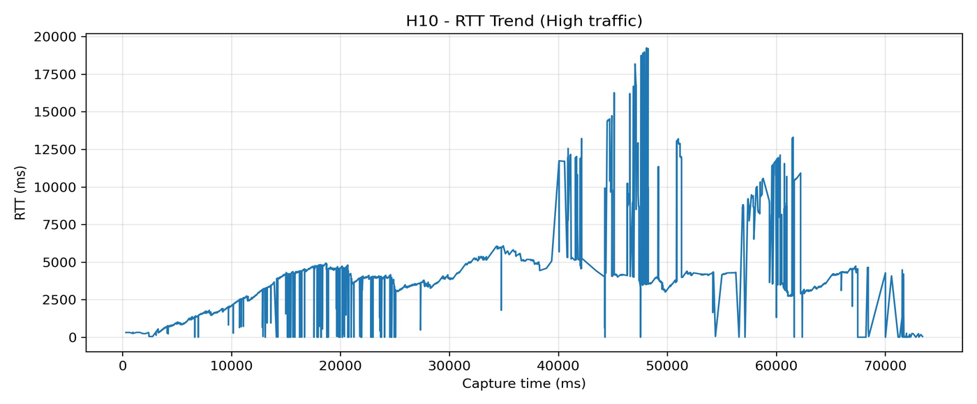
Inference. The designed worst-case: 10 streams, 60 seconds, 10 Mbps each. Average 5306 ms sustained over 74 seconds, with three clearly separated chaos phases. This is what a link that is functionally broken for interactive use looks like on a timeline.
So What Actually Causes High RTT?
Sustained queue pressure over time (bufferbloat). The #1 cause. Every multi-second average RTT in the dataset shows the same slow-ramp signature.
Bandwidth-capped medium traffic. Counter-intuitively worse than uncapped parallel traffic, because the cap defeats TCP's ability to self-regulate. M9 beat every high-traffic test on average RTT.
Tiny send buffers. More packets-per-second equals more queueing work, even on a single stream.
Parallel stream count. Matters, but surprisingly less than the above. More streams can regulate better than fewer.
Three Takeaways for Anyone New to Networking
1. RTT is dynamic, not static. Your ping time on an idle network is the floor, not the answer. Under load, that number can grow 10×, 50×, or 100×.
2. Bufferbloat is real, and you can see it. Those slow ramps in M5, M6, M7, M8, M9, H1 — that shape is a signature. Once you have seen it, you will recognise it everywhere.
3. Throughput and latency are in tension. You can optimise for one, but pushing either too hard destroys the other. Next time someone asks "what is your ping?", the correct answer is: "to where, under what load, and measured when?"
Methods Note
All tests executed with iperf3 against iperf.he.net. Packet captures taken with Wireshark on the client side. RTT samples extracted from TCP timestamp fields per flow. Plots generated in Python (matplotlib).
Written by: Naman Bhukar | 24BCE5047 | B.Tech CSE, VIT Chennai | 17 April 2026
Really well-structured writeup, Naman! The M9 finding genuinely caught me off guard 2 streams with a 15 Mbps cap beating every high-traffic test on average RTT is a great example of how intuition fails you in networking. The point about more streams sometimes producing lower RTT (H3 vs H4) is equally counterintuitive, and you explained the "why" cleanly without overcomplicating it.
Really well-structured writeup, Naman! The M9 finding genuinely caught me off guard 2 streams with a 15 Mbps cap beating every high-traffic test on average RTT is a great example of how intuition fails you in networking. The point about more streams sometimes producing lower RTT (H3 vs H4) is equally counterintuitive, and you explained the "why" cleanly without overcomplicating it.
ReplyDelete